R

What is R?
Who can use R on OSCER resources?
What version of R is available on OSCER resources?
What R packages are available on OSCER resources?
Starting R
Running R in a Job
Installing Additional R Packages
Resources

What is R?

R is a programming language used for statistical computing and graphics that is supported by the R Foundation for Statistical Computing. It is highly extensible and provides a variety of statistical and graphical techniques.

Who can use R on OSCER resources?

R is available to all OSCER users.

What version of R is available on OSCER resources?

Click here to find what version of R is installed and available on OSCER systems.

You can always get the latest information by following the steps below:

Log into the OSCER system
Type module avail R
Scroll down the list until you see the listing for R (similar to the highlighted image below)

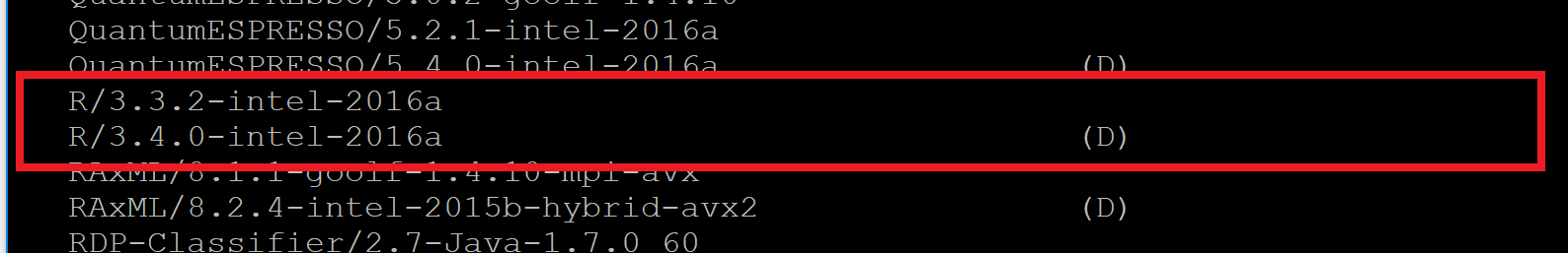
You can pick whichever version of R works best for your project, but should try to use the latest version available for best results. That is currently R/4.0.3-foss-2020b, but that will change.

What R packages are available on OSCER resources?

OSCER maintains several R packages that can be used without the need to install a local package. Follow the steps below to get the most up-to-date list:

Log into the OSCER system
Load the module for the version of R you need by typing (for example): module load R/4.0.3-foss-2020b
Then start an R session by typing: R
To obtain the list of R packages, type: library()

Starting R

Log into the OSCER system
Load the module for the version of R you need by typing (for example): module load R/4.0.3-foss-2020b
Then start an R session by typing: R

This loads R in interactive mode and will place you inside the R console. This is the place where you would install additional R packages, and run small R scripts (less than 3 minutes in duration).

NOTE: Any computational intensive work should be submitted as a job. Please refer to Running R in a Job.

Installing Additional R Packages

This section guides you through the process of installing R packages locally without root access on OSCER systems.

We highly recommend looking through the pre-installed packages to see if the package you want is already installed on OSCER systems. To do this, please refer to What R packages are available on OSCER resources?

The follow steps will guide you through the process of installing local R packages in your home directory. Please note that we do not recommend installing R packages in your scratch folder because of our autodelete policy.

In this example, we will install the package ACSWR from https://cran.r-project.org/web/packages/available_packages_by_name.html

Log into the OSCER system
Load the module for the version of R you need by typing(for example): module load R/4.0.3-foss-2020b
Start an R session by typing: R
To install the ACSWR package, type: install.packages(c("ACSWR"))
You will be prompted with the following message:
      Installing package into ‘/usr/lib64/R/library’
      (as ‘lib’ is unspecified)
      Warning in install.packages(c("ACSWR")) :
   'lib = "/usr/lib64/R/library"' is not writable
      Would you like to use a personal library instead? (y/n)
Type y and press Enter. This tells R that you will be installing the package in a local folder that you have access to (your home directory).
Next, you will be prompted with the following message:
     Would you like to create a personal library
     ~/R/x86_64-redhat-linux-gnu-library/3.3
     to install packages into? (y/n)
Type y and press Enter. This will create the folder /R/x86_64-redhat-linux-gnu-library/3.3 in your home directory.
Next, you'll get the following message asking you to choose an install source:
     --- Please select a CRAN mirror for use in this session ---
HTTPS CRAN mirror

1: 0-Cloud [https]                   2: Algeria [https]
3: Australia (Canberra) [https]      4: Australia (Melbourne 1) [https]
5: Australia (Melbourne 2) [https]   6: Australia (Perth) [https]
7: Austria [https]                   8: Belgium (Ghent) [https]
9: Brazil (PR) [https]              10: Brazil (RJ) [https]
11: Brazil (SP 1) [https]            12: Brazil (SP 2) [https]
13: Bulgaria [https]                 14: Canada (BC) [https]
15: Canada (MB) [https]              16: Canada (NS) [https]
17: Chile 1 [https]                  18: Chile 2 [https]
19: China (Beijing) [https]          20: China (Hefei) [https]
21: China (Guangzhou) [https]        22: China (Lanzhou) [https]
23: China (Shanghai 1) [https]       24: China (Shanghai 2) [https]
25: Colombia (Cali) [https]          26: Czech Republic [https]
27: Denmark [https]                  28: East Asia [https]
29: Ecuador (Cuenca) [https]         30: Ecuador (Quito) [https]
31: Estonia [https]                  32: France (Lyon 1) [https]
33: France (Lyon 2) [https]          34: France (Marseille) [https]
35: France (Montpellier) [https]     36: France (Paris 2) [https]
37: Germany (Erlangen) [https]       38: Germany (Göttingen) [https]
39: Germany (Münster) [https]        40: Greece [https]
41: Iceland [https]                  42: India [https]
43: Indonesia (Jakarta) [https]      44: Iran [https]
45: Ireland [https]                  46: Italy (Padua) [https]
47: Japan (Tokyo) [https]            48: Japan (Yonezawa) [https]
49: Korea (Seoul 1) [https]          50: Korea (Ulsan) [https]
51: Malaysia [https]                 52: Mexico (Mexico City) [https]
53: New Zealand [https]              54: Norway [https]
55: Philippines [https]              56: Serbia [https]
57: Singapore (Singapore) [https]    58: Spain (A Coruña) [https]
59: Spain (Madrid) [https]           60: Sweden [https]
61: Switzerland [https]              62: Taiwan (Chungli) [https]
63: Turkey (Denizli) [https]         64: Turkey (Mersin) [https]
65: UK (Bristol) [https]             66: UK (London 1) [https]
67: USA (CA 1) [https]               68: USA (IA) [https]
69: USA (IN) [https]                 70: USA (KS) [https]
71: USA (MI 1) [https]               72: USA (NY) [https]
73: USA (OH) [https]                 74: USA (OR) [https]
75: USA (TN) [https]                 76: USA (TX 1) [https]
77: Vietnam [https]                  78: (HTTP mirrors)
Type 1 and press Enter.
At this point, the system will attempt to download the source package and install it in your home directory.
Upon completion, you have successfully installed the ACSWR package in the following location in your home directory: /R/x86_64-redhat-linux-gnu-library/3.3/ACSWR

Running R in a Job

The sample code below shows how to submit an R job via the batch script. If you are not familiar with OSCER's job scheduler or submitting batch scripts, please refer to the following tutorials first:

Steps to submit an R job:

Step 1: Create a sample R job script called helloworld.r and insert the following line of code:

print("hello world")

Step 2: Create a batch submission file called r_batch.sh and insert the following lines of code:

#!/bin/bash
#
#SBATCH --partition=normal
#SBATCH --ntasks=1
#SBATCH --mem=1024
#SBATCH --output=r_output_%J.txt
#SBATCH --error=r_error_%J.txt
#SBATCH --time=12:00:00
#SBATCH --job-name=jobname
#SBATCH --mail-user=youremailaddress@yourinstitution.edu
#SBATCH --mail-type=ALL
#SBATCH --chdir=/home/yourusername/directory_to_run_in
#
#################################################
module load R/4.0.3-foss-2020b
Rscript helloworld.r > output.txt

In summary, the batch script asks for 1 CPU core along with 1024MB of memory for 12 hours. If your job expeccts to run on multiple cores in parallel, please specify that in '--ntasks=' instead. If it can run on all cores in a node (currently 20 or 24 on Schooner copmute nodes), please replace '--ntasks=1' with '--exclusive', to request the entire node, and prevent other jobs from running there at the same time.

Once the job starts, it runs the commands:

module load R/4.0.3-foss-2020b
Rscript helloworld.r > output.txt

on whatever compute node the job is running on. The first command prepares to run R. And the second actually runs the R script helloworld.R and places the output in the file output.txt. You can change these to whatever values are appropriate for you.

Note: Any large output should go to your /scratch space as your home directory is modest (currently 20GB). /scratch is never backed up and is subject to file purging/cleaning of older files (files older than 2 weeks).

Step 3: Submit the batch job by typing sbatch r_batch.sh

Step 4: Upon successful completion of the job, you will find three new files in your directory: output.txt, r_output_<SLURM_jobID>.txt and r_error_<SLURM_jobID>.txt. The '%J' will be replaced by the SLURM jobID, therefore avoiding overwriting files from older jobs.

Step 5: If the job ran successfully you should see the results in output.txt. If your R job produces other output files, they will be created in that directory as well.

Resources

Additional support references can be found here:

R

Quick Links

Using R Packages on OSCER Systems

Table of Contents